GITT measures voltage responses and infers diffusivity through a model
The galvanostatic intermittent titration technique (GITT) applies a constant current for a specified duration near a given composition, interrupts the current, and records the ensuing relaxation before repeating the sequence. Each pulse produces a small change in the working electrode's average lithium content while establishing concentration gradients within the material. The rest period captures the voltage response as the system approaches a more uniform state. By combining transient measurements with near-equilibrium potential measurements, Weppner and Huggins linked electrode kinetics with thermodynamic properties. [1]
When the classical model applies, GITT yields the chemical diffusion coefficient, D̃, which describes the macroscopic relaxation of a compositional perturbation and incorporates both transport kinetics and the thermodynamic driving force. It cannot be directly equated with self-diffusivity obtained from tracer measurements or molecular-dynamics mean-squared displacements. For a porous composite electrode whose particle geometry, active area, or rate-limiting process remains uncertain, a more appropriate description is an apparent chemical diffusion coefficient under the stated model and test conditions. Values reported in different studies are meaningfully comparable only when their definitions, temperatures, compositions, and geometric conventions are consistent. [1,2]
The standard equations require local linearity and a short-time approximation
From surface concentration to the voltage slope
Consider a planar, single-phase material with an initially uniform concentration and an approximately constant local diffusivity. When lithium enters through the same surface at a constant molar flux J, the semi-infinite solution of Fick's second law predicts a surface concentration change proportional to √t. Let c denote volumetric molar concentration, c0 the initial concentration, and cs the surface concentration. Neglecting side reactions and assuming one electron per lithium atom, J = I/(FS), where I is the positive magnitude of the lithiation current, F is the Faraday constant, and S is the effective reaction area carrying that flux. [1,2]

If the equilibrium potential Eeq can be linearized over the composition change within a pulse, and the voltage slope in the selected interval is dominated by solid-state diffusion, concentration changes can be converted to potential changes through dEeq/dc. Defining k = dE/d√t gives the slope-based expression below. The units of k are V s−1/2; use consistently signed derivatives, or consistently take their magnitudes before squaring.

This derivation does not require the material to behave as an ideal solution at every composition. It requires a local chemical diffusivity to describe the small perturbation and a locally linear potential–composition relationship. Within a single-phase region, substantial nonideality can appear as composition-dependent thermodynamic slopes and D̃. If one pulse spans too wide a composition interval, replacing those variations with constants becomes unreliable.
The two voltage differences must be defined separately
Let Va be the total volume of active material participating in the reaction and τ the pulse duration. Mass conservation gives the average concentration increment Δc̄ = Iτ/(FVa). Approximating the thermodynamic potential increment by ΔEs, the difference between fully relaxed potentials before and after the pulse, converts Equation (2) into the familiar voltage-ratio expression:

Here, ΔEs connects the equilibrium state before the pulse with the equilibrium state reached after the pulse and sufficient relaxation. The voltage immediately after current interruption cannot replace the latter equilibrium potential. By contrast, ΔEτ is the diffusion-related voltage change during the pulse. A corrected endpoint difference can approximate k√τ only when E is approximately linear in √t and other voltage contributions have been adequately separated. If an intermediate fitting window is used, report its actual start and end times and calculate from the slope; the voltage difference within that window must not be substituted directly for the full-pulse ΔEτ.
For active material of mass m and density ρ, Va = m/ρ. Equivalently, Va = mVm/M, where Vm is the molar volume and M is the molar mass consistent with the chosen mass definition. Conductive additives, binder, and pore volume must not be included in the active-phase volume. Using metres for Va/S and seconds for τ gives D̃ in m2 s−1; using centimetres gives cm2 s−1. The conversion is 1 cm2 s−1 = 10−4 m2 s−1.
Physical processes determine the usable fitting window
The short-time condition means that diffusion has not yet substantially sensed the finite boundaries of the material: √(D̃t) must be much smaller than the characteristic dimension L. It does not prescribe one universally short pulse for every electrode. For a slab of known thickness, L is the diffusion thickness appropriate to the boundary conditions. For approximately spherical particles, the short-time condition should be evaluated using the particle radius, not the thickness of the entire coating. At the opposite end of the timescale, the beginning of the pulse may contain current-switching transients, double-layer charging, and rapid interfacial responses. A usable window must therefore avoid these early contributions while preceding appreciable finite-size effects. [2]
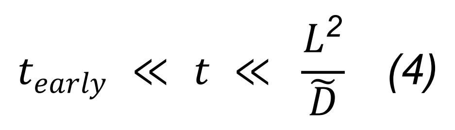
Equation (4) expresses this separation of timescales conceptually. The parameter tearly represents the time by which early non-diffusive responses have sufficiently diminished; it has no universal value. If interfacial reactions continue to dominate the voltage, deleting the first few data points will not create a diffusion-controlled regime. Even a high coefficient of determination over a narrow linear-fitting window is insufficient: shift the window to test slope stability and inspect residuals for systematic curvature. Because D̃ is initially unknown, an initial estimate can be followed by a retrospective check of the short-time condition and validation with different pulse durations, rather than a single substitution into the equation.
Geometry imposes further restrictions. Kang and Chueh compared planar, cylindrical, and spherical systems and showed that extending the semi-infinite planar solution to finite particles introduces slope deviations that grow with time. Figure 1 illustrates the shorter linear relaxation region following a longer pulse. Very small particles are therefore not necessarily better suited to conventional GITT inference: when internal diffusion is rapid, the required short-time window may have ended by the time interfacial transients subside. [2]
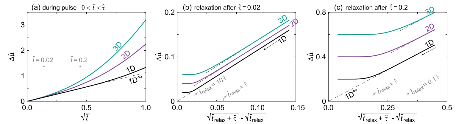
Figure 1. Effects of finite size and particle geometry on pulse responses and relaxation-analysis windows.
Major errors arise from area, polarization, and equilibrium-potential identification
Effective reaction area sets the diffusivity scale
The area S in Equation (3) cannot be chosen arbitrarily. For a dense slab, it may be the surface in contact with the electrolyte that carries the reaction. For a porous electrode, it represents the total particle surface area actually participating in lithium exchange. Electrode footprint, specific surface area measured by Brunauer–Emmett–Teller (BET) gas adsorption, and electrochemically active area generally describe different quantities. Pore wetting, binder coverage, particle contacts, and cracking can alter the relationships among them. An area value is meaningful only in the context of explicit model assumptions. [2]
For ideal spherical particles of uniform radius with fully reactive surfaces, Va/S = Rp/3. This ratio does not mean that Rp/3 should replace the radius when evaluating the short-time condition. For a particle-size distribution, explain how the chosen effective radius relates to total volume and total surface area rather than using an undefined average particle size. Equation (3) also shows directly that, with all other inputs unchanged, using twice the true S gives one-quarter of the true D̃. This is an algebraic sensitivity example, not an experimentally measured error for a particular material.
Subtracting an instantaneous drop does not remove all non-diffusive polarization
The measured voltage also contains ohmic losses, interfacial reaction overpotentials, surface-film responses, electrolyte-transport contributions, and the counter-electrode response. Subtracting a fixed IR term, where I is current and R is the equivalent resistance of the contribution being removed, corrects only the approximately instantaneous, constant component. If charge-transfer resistance changes with surface composition, it can still introduce an additional slope during the pulse. Figure 2 illustrates how a smooth voltage curve can have a slope against √t that differs from the slope produced by diffusion alone. [2]
The direction of this bias is not fixed. Additional polarization that increases the slope magnitude can lower the inferred D̃ because D̃ is inversely proportional to k2. A contribution that partially cancels the diffusion-related potential change can instead raise the inferred value. Different D values during charge and discharge therefore do not, by themselves, demonstrate intrinsically different lithium diffusivities in the two directions. Reaction overpotentials, composition paths, phase states, and counter-electrode effects should be examined first.
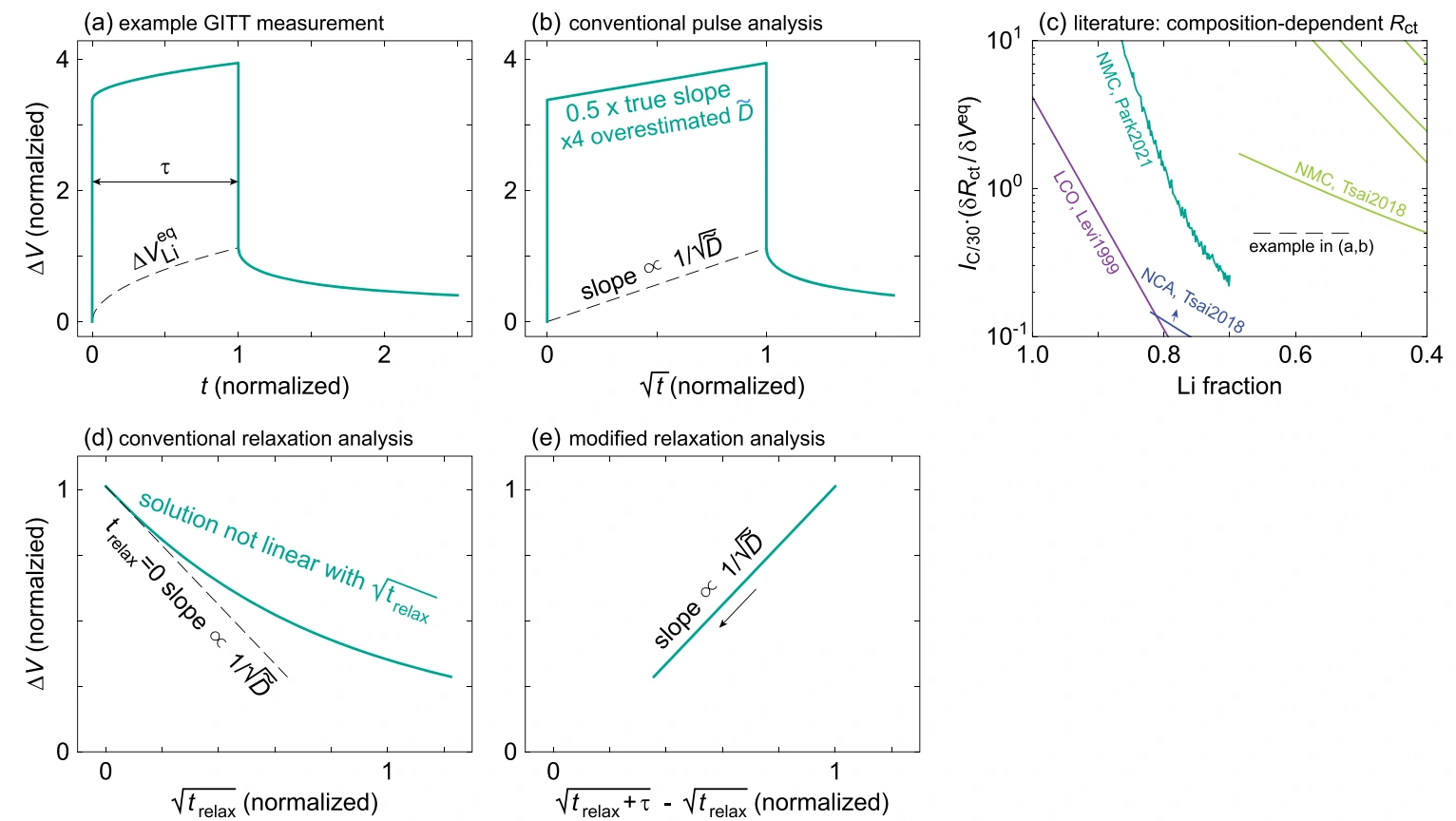
Figure 2. Voltage contributions and time-variable selection in GITT pulse and relaxation analysis.
Incomplete relaxation and low signal-to-noise ratios distort the voltage ratio
A fixed rest duration does not establish that thermodynamic equilibrium has been reached. Concentration gradients remaining from the previous pulse alter the initial conditions of the next, and residual endpoint errors propagate into ΔEs. Preliminary tests should examine late-stage voltage drift and temperature changes, then extend the rest periods at selected representative compositions to check whether ΔEs and D̃ stabilize. A small terminal dE/dt is only a supporting criterion: on a flat potential plateau, voltage is insensitive to composition changes, so apparently stable voltage does not necessarily indicate an internally uniform material.
Too little current reduces the signal-to-noise ratio of the potential change, whereas too much current can violate the small-perturbation assumption. Because D̃ has quadratic sensitivity to both ΔEs and ΔEτ, relative errors rise rapidly when the equilibrium-potential difference approaches the magnitude of drift or measurement uncertainty. Such intervals should be flagged as difficult to identify reliably, with raw curves and uncertainty information retained. Smoothing the results into a continuous D curve cannot restore the missing information.
Porous electrodes, two-phase regions, and full cells require different interpretations
The classical analytical expression is best suited to single-phase systems with well-defined geometry and boundaries, nearly uniform initial conditions, and a separable diffusion signal. In porous composite electrodes, electrolyte concentration gradients, through-thickness reaction nonuniformity, and lithium redistribution between particles must also be examined. When particle reactions are primarily controlled by interfacial exchange, the collective voltage relaxation cannot be interpreted directly as diffusion within one representative particle. In their modified experiments, Kang and co-workers measured diffusion in dense specimens and determined the equilibrium-potential relationship separately using small-particle samples, tailoring the conditions to each measurement. [2,3]
In two-phase coexistence regions, voltage may couple to nucleation, phase-boundary motion, and changing phase fractions, making a small concentration-perturbation model for a homogeneous single phase insufficient. Small ΔEs values near an equilibrium-potential plateau further destabilize voltage-ratio inference. A minimum in D near the two-phase plateau of lithium iron phosphate or a graphite staging transition therefore cannot be assigned to reduced intrinsic transport kinetics from GITT alone; structural characterization and a phase-transformation-appropriate model are needed. GITT can still record the kinetic response in these regions, but recording that response and interpreting it with a single-phase equation are distinct tasks. [2]
Half-cells are not intrinsically free of interference: polarization of the lithium-metal counter electrode can contribute to the working-electrode signal. Full-cell terminal voltage contains the potentials of both electrodes as well as transport losses, so one two-terminal voltage trace generally cannot uniquely identify the D̃ of either electrode. For material-parameter studies, consider a reference electrode, separate electrode measurements, or a coupled model constrained by independent data. For whole-cell comparisons, explicitly report the apparent response and the conditions under which it was obtained.
Relaxation analysis and numerical fitting still require validation
Analyzing voltage after current interruption can reduce interference from overpotentials present during current flow, but the relaxation curve should not be fitted arbitrarily as a linear function of √tr. Under local linearity, semi-infinite diffusion, and a constant-current pulse of finite duration, superposition of the pulse-on and pulse-off responses naturally gives the following variable. Here, tr is measured from current interruption and τ is the preceding pulse duration:

Kang and Chueh proposed using this variable to identify a linear region in the relaxation voltage, as illustrated in Figure 2e, and subsequently demonstrated the approach experimentally. [2,3] Changing the horizontal axis does not make every part of a rest period suitable for analysis: early interfacial responses, finite-size effects, and residual gradients from the previous pulse still require attention. In the limit tr ≫ τ, u approaches τ/(2√tr); this long-time approximation must not be used interchangeably with the full expression without checking its validity.
Another approach fits the pulse and subsequent relaxation jointly to an electrochemical model that explicitly describes particle diffusion and interfacial reactions. Horner and co-workers applied such an approach within the intercalation regime of FeS2 and tested the predictive ability of the inferred parameters against independent discharge data. [4] This moves validation beyond reproducing the fitted curve to explaining data withheld from the fit. Nevertheless, complex models can exhibit parameter compensation. If area, particle size, reaction rate, and diffusivity all vary freely, a good fit does not guarantee unique parameters; independent measurements and sensitivity analysis are needed to constrain them.
A workflow from test design to reproducible results
Define the target quantity and model boundaries
First decide whether the target is the material's chemical diffusivity or the apparent kinetics of an electrode made under a fixed processing protocol. Record active-material composition, mass and density sources, particle size and its statistical definition, electrode area, loading, thickness, electrolyte, and cell configuration, together with temperature, cycling history, and current direction. Establish flagging criteria for phase-transition regions and low-signal intervals in advance so that subsequent data selection does not depend on whether the results meet expectations.
Determine pulse, rest, and sampling conditions in preliminary tests
At several representative compositions, vary pulse current, pulse duration, and rest duration independently to assess whether the potential response meets the requirements of a small perturbation, measurable signal, and separated timescales. Report both absolute current and its normalization basis; describing a test only as low-rate is not reproducible. If the rate r is expressed in h−1 and the reference capacity Qref in Ah, I = rQref is in amperes. With τ in hours, the capacity fraction changed per pulse is rτ. For example, C/20 for 10 min corresponds to approximately 0.83% of the reference capacity. This is only a charge calculation and does not establish that a material satisfies the GITT assumptions.
Retain sufficiently dense data around current switching to resolve transients and enough information during long rests to resolve late-stage drift. Record actual current, timestamps, voltage, temperature, and step boundaries, checking for range changes, missing data, and offsets in the time origin. Sampling intervals and rest-termination criteria should follow the observed signals rather than being copied unchanged from a protocol for another material.
Retain fitting details and quality decisions for every pulse
Segment the raw data by test step and set the appropriate time origin at pulse onset or current interruption. Preserve candidate fitting windows, slopes, residuals, and potentials before and after relaxation. After calculating D̃, check the short-time condition and compare results obtained by shifting the fitting window, shortening the pulse, or extending the rest. Flag points for which no linear region exists, the equilibrium-potential difference cannot be resolved reliably, or the parameter is highly sensitive to the chosen window, and report the reason rather than only a number.
Relate software outputs to physical validity criteria
In a NEWARE battery testing system, constant-current and rest steps can be configured according to the preliminary test plan while retaining the raw data needed for independent recalculation. The official NEWARE BTS tutorial demonstrates exporting specific capacity and diffusion coefficients from GITT data in BTSDA using version 8.0.1.492. In practice, verify the equations, parameter definitions, units, and point-selection rules used by the installed software version. Do not assume that the software automatically establishes effective reaction area, equilibrium, or the presence of a two-phase region.
For publication or material comparisons, report D̃ as a function of composition or capacity together with representative pulse and relaxation curves, the equation used, the basis for area or effective particle size, fitting windows, relaxation criteria, and variability between replicate specimens. To claim that a modification improves intrinsic material diffusion, additionally rule out explanations such as changes in particle size, improved wetting, or altered reaction area, and test whether the inferred parameters describe data under independent operating conditions.
Build a GITT workflow with NEWARE
NEWARE brings test execution and data analysis into a connected laboratory workflow. The CT/CE-4000 series combines charge/discharge and pulse testing with BTS software, while compatible environmental test chambers support temperature-controlled studies. For GITT, this provides a practical platform for implementing pulse/rest protocols and comparing responses under defined conditions. The official GITT export tutorial lists the CT-4008Q-5V100mA among its applicable instruments; the appropriate configuration should still be selected against the actual pulse current, voltage signal, and required recording interval. The software workflow described above then supports report export for subsequent interpretation and comparison. Figure 3 shows the rack configuration presented on the CT-4008Q-5V100mA-124 product page.

Figure 3. Rack configuration shown on the NEWARE CT-4008Q-5V100mA-124 product page.
Planning a GITT study? Contact NEWARE with your cell format, voltage window, expected pulse-current range, channel count, and temperature requirements to discuss a suitable tester and chamber configuration. Matching the equipment to the experiment helps turn the method into a repeatable testing workflow, while the model checks in this article remain essential to interpreting the results.
Conclusion
The scientific value of GITT lies in establishing testable relationships among composition, potential response, and transport. The credibility of an inferred diffusivity depends on whether the model represents the actual system: whether a short-time diffusion window exists, the thermodynamic potential change is reliable, effective area is defined, and non-diffusive processes are separated. In porous electrodes, two-phase regions, and full cells, distinguish material chemical diffusivity from apparent kinetic parameters according to the strength of the evidence. Explicit assumptions, raw curves, and validation provide stronger support for mechanistic conclusions than a smooth diffusivity curve alone.
References
[1] Weppner W, Huggins R A. Determination of the Kinetic Parameters of Mixed-Conducting Electrodes and Application to the System Li3Sb. Journal of The Electrochemical Society, 1977, 124(10): 1569–1578. https://doi.org/10.1149/1.2133112
[2] Kang S D, Chueh W C. Galvanostatic Intermittent Titration Technique Reinvented: Part I. A Critical Review. Journal of The Electrochemical Society, 2021, 168(12): 120504. https://doi.org/10.1149/1945-7111/ac3940
[3] Kang S D, Kuo J J, Kapate N, Hong J, Park J, Chueh W C. Galvanostatic Intermittent Titration Technique Reinvented: Part II. Experiments. Journal of The Electrochemical Society, 2021, 168(12): 120503. https://doi.org/10.1149/1945-7111/ac3939
[4] Horner J S, Whang G, Ashby D S, Kolesnichenko I V, Lambert T N, Dunn B S, Talin A A, Roberts S A. Electrochemical Modeling of GITT Measurements for Improved Solid-State Diffusion Coefficient Evaluation. ACS Applied Energy Materials, 2021, 4(10): 11460–11469. https://doi.org/10.1021/acsaem.1c02218