1. Kinetic information in the voltage response to current interruption
During charging, the terminal voltage reflects the combined effects of electron and ion transport, interfacial reactions and concentration distributions. When the current stops, these contributions relax at different rates, producing an initial rapid voltage change followed by a slower response. By repeatedly inserting short interruptions into constant-current operation, ICI provides diagnostic information at different charge states and helps track how battery kinetics evolve with aging. [1,2]
1.1 Two components of voltage relaxation
Figure 1 illustrates this response. After the current is interrupted at approximately 300 s, the voltage first drops rapidly (arrow a) and then decreases more slowly (arrow b). It rises again when the current resumes at approximately 301 s. The rapid change includes the removal of the ohmic voltage drop and the relaxation of fast polarization processes; the subsequent change reflects continuing relaxation. [3]
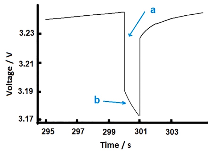
Figure 1. Rapid voltage change and slower relaxation after current interruption
Within a diffusion-controlled analysis interval, the voltage change is approximately linear with the square root of time. Fitting this interval with a straight line and dividing its intercept and slope by the magnitude of the current immediately before interruption gives R and k, respectively. R is an effective resistance that includes ohmic and fast polarization contributions, expressed in Ω. The coefficient k describes the strength of the diffusion-related voltage response, expressed in Ω·s−1/2. The following sections show how to extract both parameters from the voltage data. [1,3]
1.2 Test sequences for ICI and GITT
The galvanostatic intermittent titration technique (GITT) typically combines short current pulses with longer rest periods, allowing the voltage to approach equilibrium during rest. ICI maintains largely continuous constant-current charging or discharging, with interruptions lasting a few seconds. Analyzing these brief responses provides repeated measurements of kinetic parameters at different charge states throughout the test. [1]
Figure 2 links the test sequences to their analysis. The upper panels, a → c → e, show the ICI current sequence, the voltage response over time and the voltage plotted against the square root of time. The lower panels, b → d → f, show the corresponding GITT procedure. The orange lines indicate fitted slopes over selected intervals. This source experiment uses 10 s ICI interruptions; Section 2 presents a separate example with 5 s interruptions.
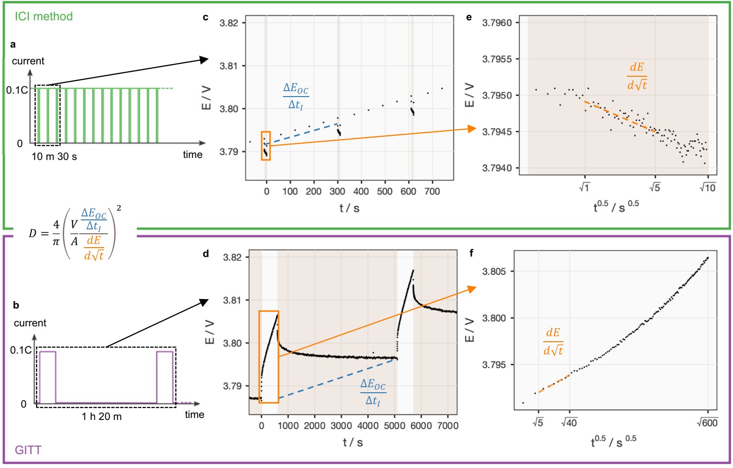
Figure 2. ICI and GITT test sequences, voltage responses and square-root-of-time analysis
Figure 2 also gives a relationship for calculating the chemical diffusion coefficient, D. Combining the voltage-response slope with the change in quasi-equilibrium potential and the material geometry allows D to be calculated within the corresponding diffusion model. D is usually expressed in cm2/s or m2/s and describes the rate of ion diffusion. R and k are extracted directly from the interruption response and are useful for tracking changes in battery kinetics throughout a test.
2. Implementing ICI with NEWARE testing systems
2.1 Current control and data acquisition
An ICI test requires the battery testing system to perform three tasks: apply a stable constant current, briefly switch to zero current, and record voltage and current around each transition. In his publicly available ICI implementation guide, method developer Matthew J. Lacey explicitly lists NEWARE among the equipment brands that have successfully been used for ICI measurements. [4]
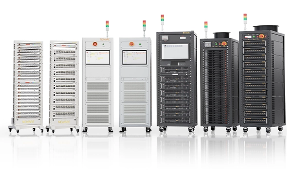
Relevant configurations of the NEWARE CT-9000 series support data recording at up to 1000 Hz, enabling voltage acquisition during brief current interruptions. For ICI, the recording interval can be selected to suit the analysis window, together with a current range appropriate for the test current. Current control and voltage sampling then provide the inputs needed for fitting. The series uses BTS 9.x software for test-step configuration and data recording.
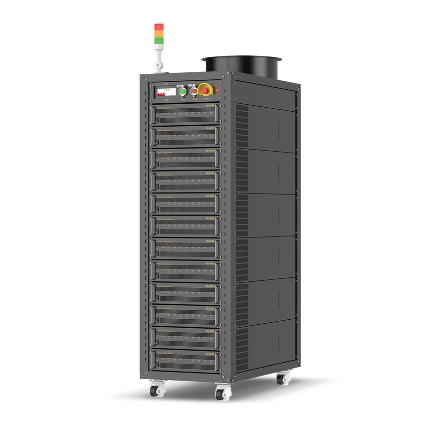
Figure 3. NEWARE CT-9000 series cabinet battery testing system
In these measurements, the sampling frequency determines the density of recorded points, while the current response time describes how quickly the system switches between steps. Recording measured current together with timestamps helps locate the interruption onset accurately. The continuous voltage record is then used to calculate R and k.
2.2 An ICI measurement explained through test steps and curves
Lacey's published example repeats 5 min of constant-current charging at C/10 followed by a 5 s interruption, recording the voltage every 0.2 s during the interruption. [4] For an illustrative 5 Ah cell with a 4.2 V upper charging limit, set the current to 0.5 A, charge for 300 s and then rest for 5 s. Figures 4 and 5 use recreated BTS 8.0 and BTSDA interfaces to connect the settings, curves and simulated records. BTS 8.0 supports series such as CT-4000 and CT-8000; implement the same current/rest sequence in BTS 9.x for CT-9000 systems.
In Figure 4, Step 1 is constant-current charging, Step 2 is rest, and Step 3 returns to Step 1 for three repetitions of the charge/rest pair. The 0.2 s recording interval provides voltage measurements during each rest period. This is a short charge/rest example. For full cycling, configure voltage-triggered branching to leave the charging loop at the upper limit and proceed to discharge or End.
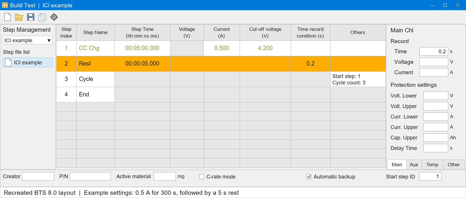
Figure 4. ICI step settings in a recreated BTS 8.0 interface
Figure 5 shows the data around one interruption. The dashed blue line is the current: it drops from 0.5 A to 0 A at a total test time of 300 s and resumes at 305 s. The red voltage curve falls rapidly at first and then more slowly. The selected records on the right correspond to the curve on the left. Total times of 301 s and 304 s are 1 s and 4 s after interruption, respectively.
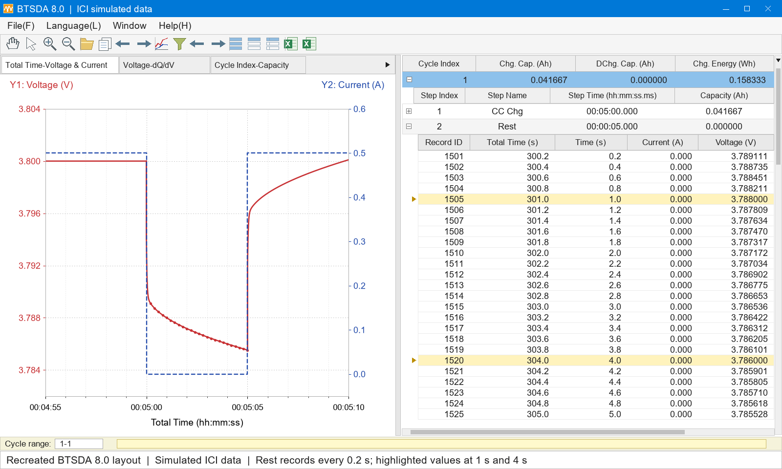
Figure 5. Simulated ICI curves and records in a recreated BTSDA 8.0 interface
After exporting the records, use 300 s as the interruption onset and convert total test time to elapsed time t after interruption. Calculate the voltage change and fit it against the square root of time to obtain R and k. The next section uses the same data from Figure 5 to explain the calculation.
3. Calculating R and k from interruption data
3.1 Defining the time origin and voltage-change direction
Consider an interruption during charging. Define the instant at which the current actually stops as t = 0, the voltage immediately before interruption as U0, and the subsequent voltage as U(t). Since the voltage typically falls after charging is interrupted, define the voltage change as:

U0 can be taken as the average voltage over a short, stable interval immediately before interruption to reduce sampling noise. For an interruption during charging, the voltage decrease is U0 − U(t); for an interruption during discharging, the voltage increase is U(t) − U0. In both cases, use the magnitude of the current before interruption to calculate R and k.
3.2 Plotting against the square root of time
Select an appropriate interval from the interruption data, convert each time point t to √t, and perform a linear fit with √t on the horizontal axis and ΔU on the vertical axis:

Here, a is the intercept extrapolated to √t = 0, expressed in V, and b is the slope, expressed in V·s−1/2. Dividing each by the magnitude of the current before interruption gives:

First identify an approximately linear interval on the ΔU versus √t plot. Fit all sampled points in that interval to obtain the intercept a and slope b. Record the fitting interval together with R and k so that repeated measurements under the same test conditions can be compared, and apply the same procedure to subsequent interruptions.
3.3 A worked numerical example
Using the simulated data in Figure 5, the current before interruption is 0.5 A and U0 is 3.800 V. Take two representative points: 3.788 V at 1 s after interruption and 3.786 V at 4 s. The corresponding voltage changes are 12 mV and 14 mV, and the square roots of time are 1 s1/2 and 2 s1/2. These two points make the slope and intercept calculation easy to follow.
The slope and intercept calculated from these points are:


Dividing by 0.5 A gives:


The simulated data give an effective resistance of 20 mΩ and a diffusion resistance coefficient of 4 mΩ·s−1/2. A linear fit to all 21 simulated points in the 1–5 s interval gives the same results. Repeating this calculation for each interruption produces a sequence of R and k values across the test.
The calculation follows a clear sequence: locate the interruption onset, calculate the voltage change, take the square root of time, fit a straight line, and divide the intercept and slope by the current magnitude.
4. Tracking battery changes with R and k curves
Associate the R and k values from each interruption with the corresponding capacity, voltage or state of charge (SOC) to build parameter curves across charging and discharging. Overlaying the curves for a fresh cell and different aging stages shows where changes occur and whether they continue to develop with cycling.
Under the same test conditions, an overall increase in R indicates a higher effective resistance. A localized increase helps identify the charge-state range in which the change occurs. Changes in k reflect changes in the diffusion-related voltage response and can be examined alongside voltage curves, capacity fade and material characterization.
The terminal voltage of a commercial full cell combines contributions from both electrodes and other internal processes. R and k curves help locate regions of change, while electrode characterization and modeling help explain their origins. Together, these measurements connect changes in performance to the underlying mechanisms.
When comparing different aging stages, use consistent temperatures, test procedures and SOC calculations, and record the actual current. SOC can be normalized to the available capacity measured at each stage. State whether the C-rate is based on nominal capacity or the available capacity at that stage, so that the curves have a clear basis for comparison.
5. Research applications of ICI
5.1 Aging characterization of commercial cells
Geng et al. applied ICI to aging characterization of commercial lithium-ion batteries. For the cells studied, they observed changes in effective resistance and the diffusion resistance coefficient as capacity faded, and discussed repeatability and measurement requirements. [2] Capacity testing shows how much charge a cell can still store; ICI adds information about its kinetics at different states, extending aging assessment beyond a single capacity-retention value.
Yin et al. applied ICI to commercial 21700 cells and combined the measurements with a battery model. The study used cells with nickel–cobalt–aluminum oxide (NCA) cathodes and graphite anodes at 20 °C. Reference performance tests were performed every 100 cycles, using 10 min at a constant current of 0.48 A followed by a 1 s interruption, with data recorded every 0.1 s. The resulting resistance distributions as a function of capacity and cycle number were used to analyze cell aging. [3]
5.2 Local changes in NMC811 electrode kinetics
Chien et al. studied NMC811 electrodes in a three-electrode cell and extended ICI analysis to solid-state diffusion coefficients. [1] In Figure 6, panels a and b show D during charging and discharging, respectively, while panels c and d show the corresponding R values. The horizontal axis is specific capacity Q, and the colors represent cycles 6, 15, 25, 35 and 55. Comparing different colors at the same specific capacity reveals how the parameters evolve with cycling.
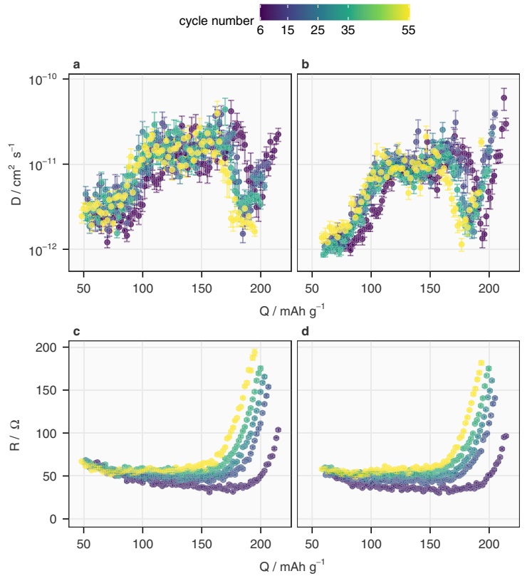
Figure 6. Diffusion coefficient and effective resistance of NMC811 electrodes during cycling
Figure 6 shows R rising broadly across the measured capacity range as cycling progresses. A more localized change appears in D: the source study identifies a decrease above 4.2 V versus Li/Li+, corresponding to about 200 mAh g−1 in cycle 6 and 180 mAh g−1 in later cycles. Comparison with the electrode potential and operando XRD measurements links this high-potential change to structural evolution in NMC811. [1]
Cell 1 was cycled at 20 mA g−1 between 3.0 and 4.3 V versus Li/Li+ in a laboratory maintained at 22 °C, using 10 s interruptions every 300 s of applied current. Figure 6 shows data for E ≥ 3.7 V. R is reported in Ω, and D represents chemical diffusion of Li ions in the NMC811 working electrode. The error bars reflect the standard deviation of the linear regression. [1]
6. Incorporating ICI into routine battery testing
ICI is useful for comparing kinetics across cells, aging stages or material formulations under consistent conditions. For example, embedding the same interruption sequence into periodic reference performance tests builds a record of R and k as a function of SOC and cycle number. This provides a practical implementation route for laboratories that already run charge–discharge tests.
For these comparisons, keep temperature, charge or discharge direction, and current settings consistent, and apply the same rule for selecting the linear fitting interval. Clear voltage responses and repeatable fits provide the basis for a reliable long-term parameter record.
ICI also complements other methods. Electrochemical impedance spectroscopy (EIS) provides information in the frequency domain, while GITT provides more complete equilibrium information and supports diffusion analysis. Relating these measurements to ICI curves helps explain battery behavior at different charge states and aging stages.
For users of NEWARE systems, the equipment executes the constant-current and interruption steps and records current, voltage and time. A data-processing program extracts each response, performs the fits and generates R and k curves. Incorporating this workflow into reference performance testing adds a continuing record of battery kinetics alongside capacity measurements.
References
[1] Chien, Y.-C., Liu, H., Menon, A. S., Brant, W. R., Brandell, D. & Lacey, M. J. Rapid determination of solid-state diffusion coefficients in Li-based batteries via intermittent current interruption method. Nature Communications 14, 2289 (2023).
[2] Geng, Z., Thiringer, T. & Lacey, M. J. Intermittent Current Interruption Method for Commercial Lithium-Ion Batteries Aging Characterization. IEEE Transactions on Transportation Electrification 8(2), 2985–2995 (2022).
[3] Yin, L., Geng, Z., Chien, Y.-C., Thiringer, T., Lacey, M. J., Andersson, A. M. & Brandell, D. Implementing intermittent current interruption into Li-ion cell modelling for improved battery diagnostics. Electrochimica Acta 427, 140888 (2022).
[4] Lacey, M. J. Intermittent current interruption (ICI). Public technical guide by the method developer, Implementation section. Accessed October 29, 2026.