DRT Explained: How Relaxation Time Analysis Reveals Battery Impedance Processes

Full-cell structure and impedance origin

A lithium-ion full cell contains a graphite anode, cathode active material, current collectors, electrolyte, and separator. During charge and discharge, electrons move through the external circuit while Li⁺ migrates through the electrolyte, interfacial films, and active-material particles. Because each conduction, reaction, and diffusion step can add impedance, a full-cell structural view is a useful starting point before reading DRT peaks.

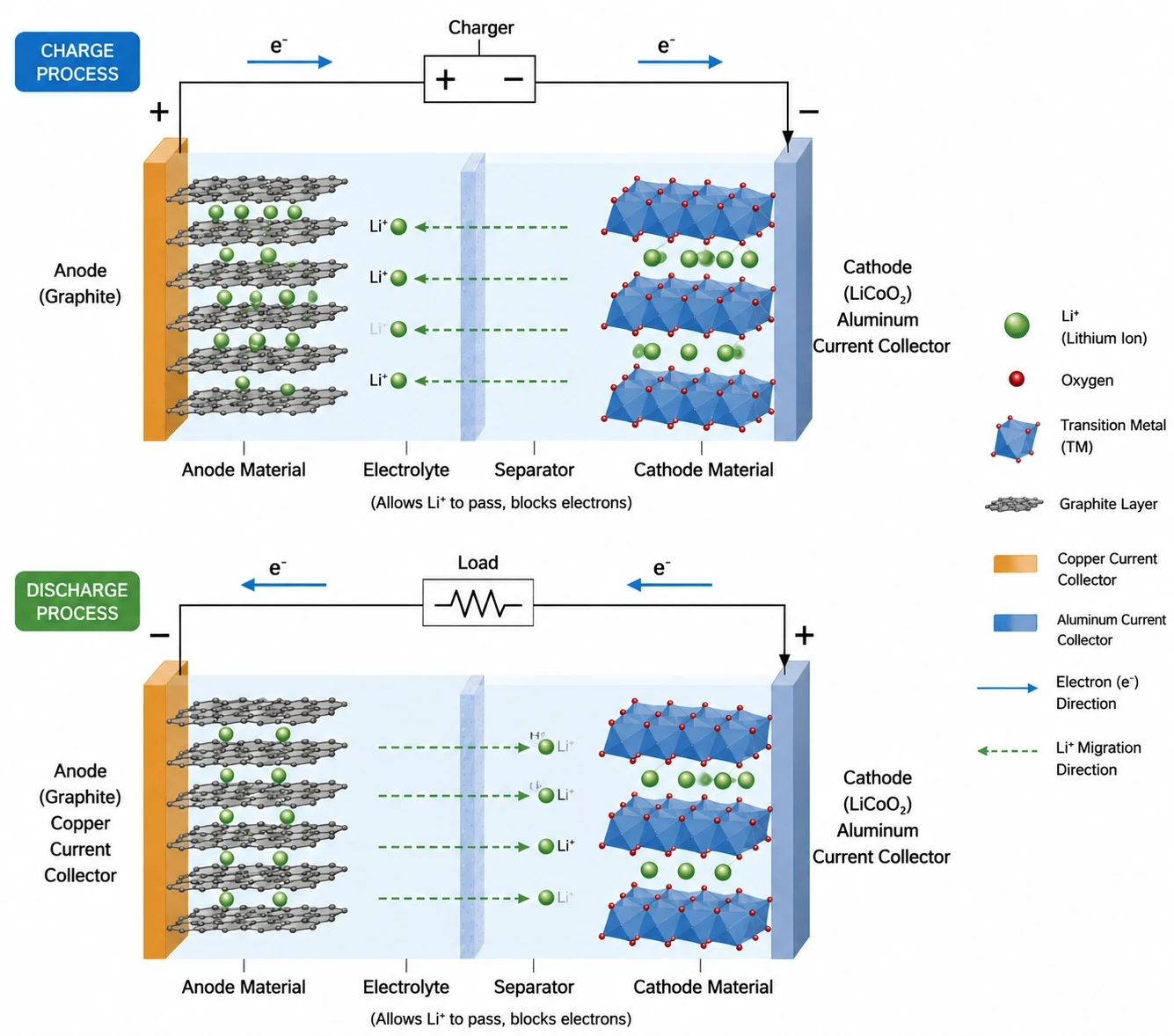
Figure 1. Lithium-ion full-cell structure during charge and discharge, showing electron flow and Li⁺ migration between graphite anode and cathode.

Equivalent circuit before DRT analysis

Before discussing the data-processing workflow, it is helpful to look at the equivalent-circuit picture. In EIS interpretation, the battery is often represented by an ohmic resistance plus several distributed interfacial, kinetic, and diffusion-related elements. This does not mean the battery literally contains these components; rather, the circuit is a compact way to describe processes that relax over different time scales.

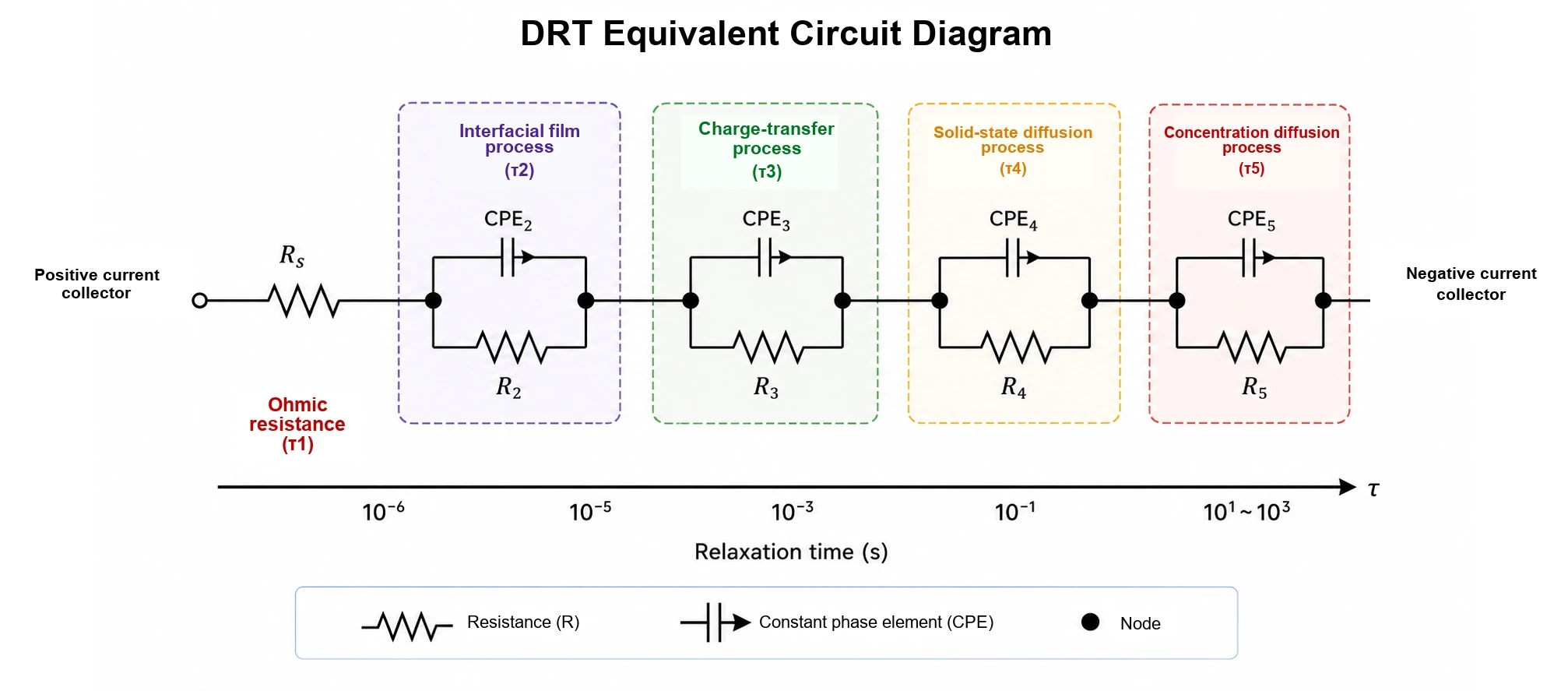
Figure 2. Equivalent-circuit interpretation of typical battery impedance processes, arranged by relaxation time.

From EIS to DRT

EIS measures the battery response to a small AC perturbation over frequency, usually under an approximately linear and time-invariant condition. Several electrochemical processes may overlap in a Nyquist plot. DRT remaps the impedance response onto relaxation time τ, so fast processes appear at small τ and slow processes appear at large τ.

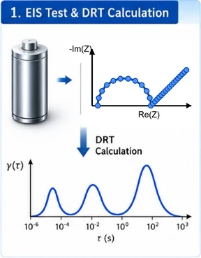
Figure 3. EIS data can be transformed into DRT peaks on a relaxation-time axis, separating overlapping impedance responses.

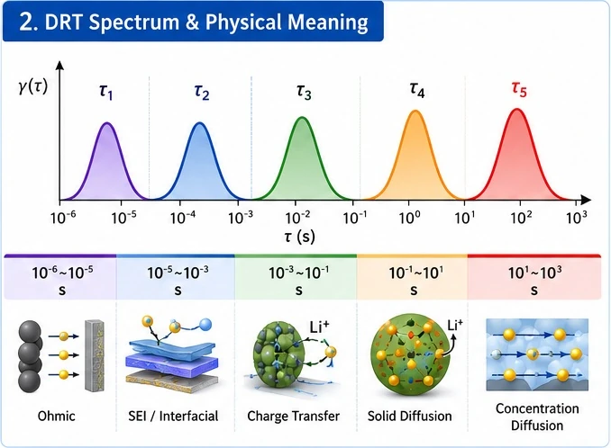
Figure 4. Physical meaning of common DRT peak regions: ohmic response, interfacial films, charge transfer, solid-state diffusion, and concentration diffusion.

Physical meaning of τ₁-τ₅

Peak assignment depends on chemistry, temperature, state of charge, cycling history, frequency window, and numerical regularization. As a practical guide, τ₁ is often close to the high-frequency ohmic/contact region; τ₂ reflects interfacial films; τ₃ reflects charge-transfer kinetics; τ₄ reflects solid-state diffusion; and τ₅ reflects slower concentration diffusion. These assignments should be treated as physically informed hypotheses, not automatic labels.

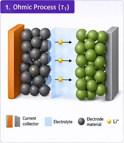
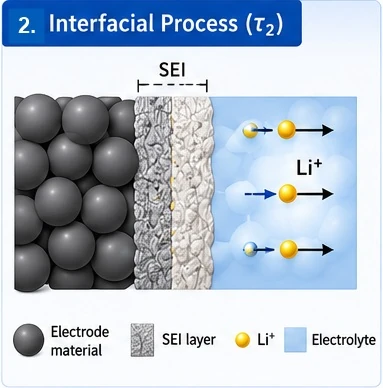
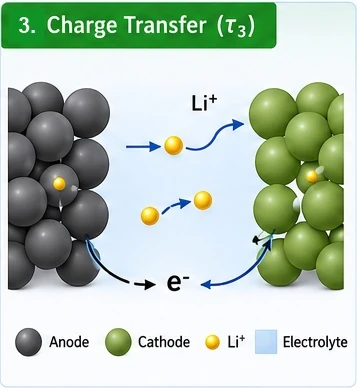
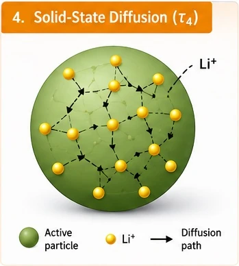
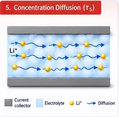
Figure 5. Multi-panel DRT process gallery: τ₁ ohmic response, τ₂ interfacial film response, τ₃ charge-transfer response, τ₄ solid-state diffusion, and τ₅ concentration diffusion.

Process-level interpretation

τ₁: ohmic response

Ohmic response generally appears near 10⁻⁶-10⁻⁵ s and reflects rapid electronic/ionic conduction, current-collector pathways, tabs, welds, and contact resistance.

τ₂: interfacial film response

Interfacial film response often occurs around 10⁻⁵-10⁻³ s and is associated with SEI/CEI layers and electrode-electrolyte contact.

τ₃: charge-transfer response

Charge transfer is commonly found around 10⁻³-10⁻¹ s. It describes how easily lithium ions and electrons complete electrochemical reactions at the interface.

τ₄: solid-state diffusion

Solid-state diffusion often appears around 10⁻¹-10¹ s and reflects lithium-ion migration inside active-material particles.

τ₅: concentration diffusion

Concentration diffusion appears at longer time scales, often near 10¹-10³ s. It reflects electrolyte or pore-scale concentration gradients and mass-transport polarization.

Common DRT analysis figures in the literature

Battery DRT papers commonly present results in four forms: raw EIS-to-DRT comparison, fresh/aged or condition-to-condition DRT spectra, stacked DRT maps across SOC or temperature, and peak fitting with process assignment. The figure below redraws these common analysis patterns as an original schematic summary rather than copying journal figures.

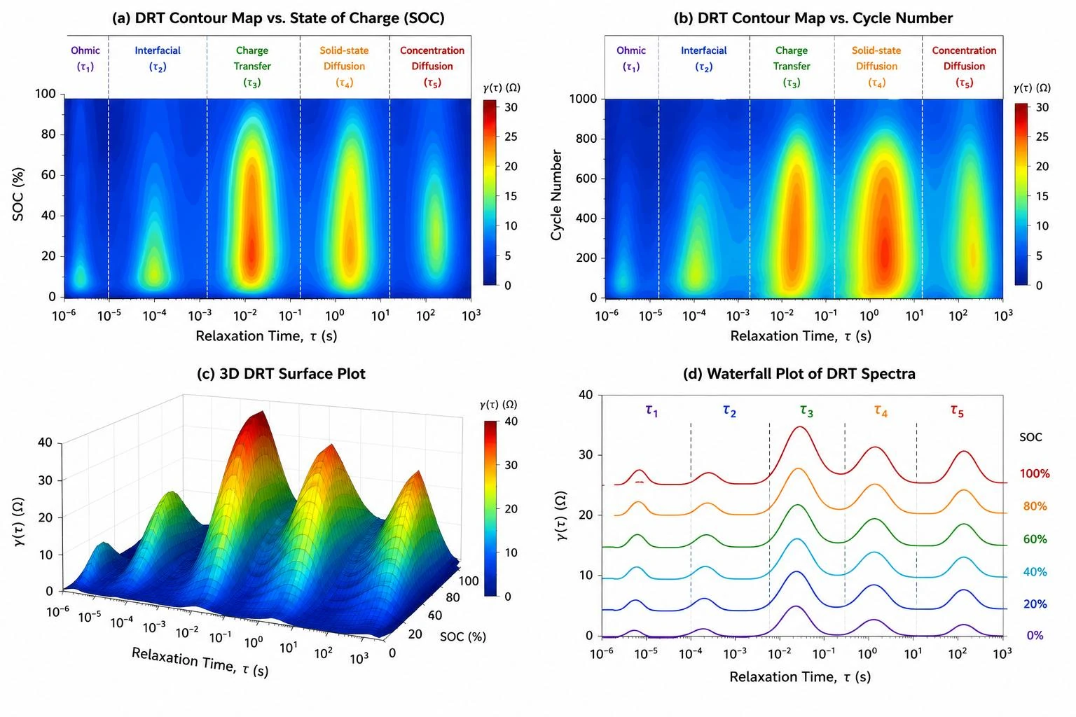
Figure 6. Original schematic summary of common DRT analysis plots in battery impedance papers: EIS-to-DRT interpretation, aging comparison, operating-condition DRT map, and peak fitting with process assignment.

Mathematical basis of DRT

The standard DRT model treats measured impedance as a superposition of many parallel RC-like relaxation processes. In continuous form, the impedance can be written as:

Here R∞ is the ohmic resistance and γ(ln τ) is the DRT function. A narrow peak in γ(ln τ) behaves like a distinct relaxation process, while a broad peak usually indicates a distributed or non-ideal process such as porous-electrode transport or heterogeneous interfaces.

If the high-frequency region contains inductive behavior, the model can include an inductance term:

Regularization, uncertainty, and data quality

Recovering γ(ln τ) from EIS data is an inverse problem. Direct inversion is ill-conditioned: small measurement noise can create artificial oscillations or split one physical process into several false peaks. DRT tools therefore use regularization, commonly Tikhonov regularization or Bayesian ridge regression.

Bayesian DRT methods can estimate a credibility interval for γ(τ). A narrow interval indicates that the peak is better supported by the data, while a wide interval warns that the apparent feature may depend strongly on noise, frequency coverage, or the regularization setting.

Before assigning peaks to battery processes, the EIS spectrum should also pass basic consistency checks. Hilbert-transform or Kramers-Kronig-style checks are often used to evaluate whether the spectrum is compatible with linear, causal, and stable impedance behavior.

Key symbols used in the equations

Practical use and interpretation rules

· Diagnose aging sources: separate resistance growth from interfacial, kinetic, and diffusion limitations.

· Compare cells or materials: detect process-level differences even when capacity values look similar.

· Track operating effects: observe how temperature, SOC, and rate shift DRT peaks.

· Avoid overinterpretation: validate DRT assignments with EIS quality, equivalent-circuit fitting, electrochemical data, and materials evidence.

References for the DRT method

· Wan, T. H.; Saccoccio, M.; Chen, C.; Ciucci, F. Influence of the Discretization Methods on the Distribution of Relaxation Times Deconvolution: Implementing Radial Basis Functions with DRTtools. Electrochimica Acta 184, 483-499 (2015).

· Ciucci, F.; Chen, C. Analysis of Electrochemical Impedance Spectroscopy Data Using the Distribution of Relaxation Times: A Bayesian and Hierarchical Bayesian Approach. Electrochimica Acta 167, 439-454 (2015).

· Effat, M. B.; Ciucci, F. Bayesian and Hierarchical Bayesian Based Regularization for Deconvolving the Distribution of Relaxation Times from Electrochemical Impedance Spectroscopy Data. Electrochimica Acta 247, 1117-1129 (2017).

· Liu, J.; Wan, T. H.; Ciucci, F. A Bayesian View on the Hilbert Transform and the Kramers-Kronig Transform of Electrochemical Impedance Data. Electrochimica Acta 357, 136864 (2020).